Biomol2Clust
Tool to cluster docked poses, structural states of ligands/peptides, and conformational variants of biological macromolecules using machine learning
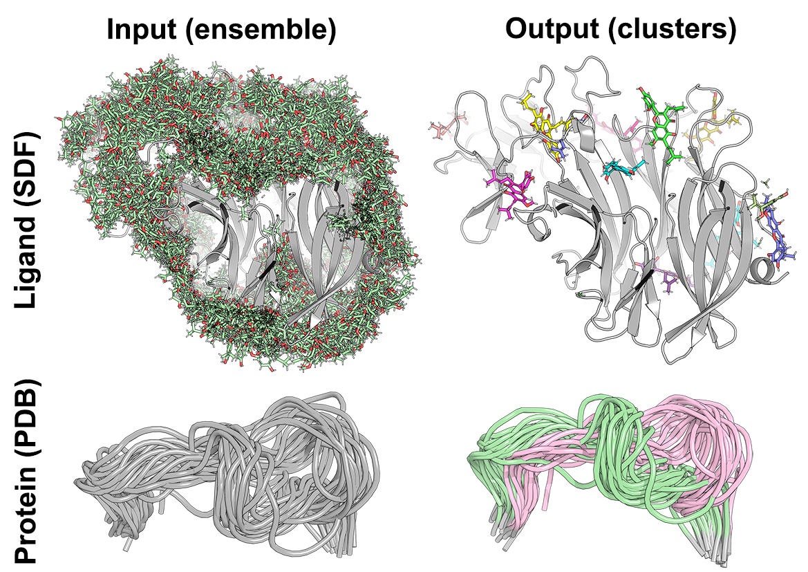
Biomol2Clust is a Python3 script to assist cluster analysis of biological molecules using machine learning. The new tool is easy-to-use and has a broad application in a daily laboratory practice: it can be used to cluster docked poses as a post-docking analytics (e.g. to summarize results of multiple dockings into one site, or bring some sense to the results of a blind full-size structure screening) and to study structurally distinct states/conformations of peptides and protein fragments (e.g. observed during a molecular dynamics simulation).
The input ensemble of protein/ligand configurations can be provided as a single SDF file (i.e. ligands in MOL format as one SDF library) or as a batch of conformations in PDB format (i.e. probably, more suitable for peptides and protein fragments). In both cases, all conformations should correspond to identical entities (i.e. of the same ligand or the same protein fragment) and should implement the common coordinate space suitable for a meaningful clustering (e.g. ligands should be docked into one protein, protein conformations should be pre-aligned, see examples in the figure above). If the input conformations do not share the common coordinate space, the align=true keyword can be used to superimpose all pairs of conformations for best-fit.
The pairwise RMSD similarity matrix will be calculated from the input data (i.e. RMSD between every two conformations) and further subjected to the selected machine learning cluster analysis technique. By default, hydrogen atoms are explicitly considered for cluster analysis, and can be dismissed by adding the noh=true keyword. Biomol2Clust implements three widely used cluster analysis methods. The HDBSCAN and OPTICS are two fully automatic techniques. The HDBSCAN is known to preserve maximum data for further expert analysis by producing “thicker” clusters and minimizing the amount of outliers (i.e. unique/rare orientations). The OPTICS, on the opposite, usually produces spatially more compact and “thinner” clusters by dismissing a larger number of conformations as outliers. Finally, the DBSCAN is a manually curated technique whose output can be calibrated for a particular purpose by fine-tuning the ‘eps’ parameter.
The software is freely available for download with no login requirement.
THIS WEB-SITE/WEB-SERVER/SOFTWARE IS PROVIDED “AS IS”, WITHOUT WARRANTY OF ANY KIND, EXPRESS OR IMPLIED, INCLUDING BUT NOT LIMITED TO THE WARRANTIES OF MERCHANTABILITY, FITNESS FOR A PARTICULAR PURPOSE AND NONINFRINGEMENT. IN NO EVENT SHALL THE AUTHORS OR COPYRIGHT HOLDERS OR HARDWARE OWNERS OR WEB-SITE/WEB-SERVER/SOFTWARE MAINTEINERS/ADMINISTRATORS BE LIABLE FOR ANY CLAIM, DAMAGES OR OTHER LIABILITY, WHETHER IN AN ACTION OF CONTRACT, TORT OR OTHERWISE, ARISING FROM, OUT OF OR IN CONNECTION WITH THE WEB-SITE/WEB-SERVER/SOFTWARE OR THE USE OR OTHER DEALINGS IN THE WEB-SITE/WEB-SERVER/SOFTWARE. PLEASE NOTE THAT OUR WEBSITE COLLECTS STANDARD APACHE2 LOGS, INCLUDING DATES, TIMES, IP ADDRESSES, AND SPECIFIC WEB ADDRESSES ACCESSED. THIS DATA IS STORED FOR APPROXIMATELY ONE YEAR FOR SECURITY AND ANALYTICAL PURPOSES. YOUR PRIVACY IS IMPORTANT TO US, AND WE USE THIS INFORMATION SOLELY FOR WEBSITE IMPROVEMENT AND PROTECTION AGAINST POTENTIAL THREATS. BY USING OUR SITE, YOU CONSENT TO THIS DATA COLLECTION.
[to the top]
Download
Download the source code using a direct link, as described below.
| Biomol2Clust Copyright (C) 2020-2021 Timonina D., Sharapova Y., Švedas V., Suplatov D. This program is free software: you can redistribute it and/or modify it under the terms of the GNU General Public License as published by the Free Software Foundation, either version 3 of the License, or any later version. See the LICENSE.txt file inside the distribution package. | |
Biomol2Clust is distributed as a 'tar.gz' archive pack. In Linux, use command tar xzf file.tar.gz to extract the data (both tar and gzip utilities usually come with the Linux distribution). In Windows, you can use a free tool 7-zip to unpack the archive. The package includes the program itself, as well as examples to test-run your installation. |
| Version | Date | List of changes | Size | Link |
| 1.3 | 2021-Jan-29 | Implemented new output feature: a dedicated output file is printed describing the assignment of input conformations, referred to by IDs/names, to output clusters/outliers | 2.0 MB | [download] |
| 1.2 | 2020-Dec-30 | Significant increase in computational efficiency due to utilization of all CPU cores when calculating pairwise RMSD similarity matrix. The -noh option added to dismiss hydrogen atoms when calculating pairwise RMSD between two conformations. For each cluster, a representative ("central") configuration is now printed to a separate file. |
2.0 MB | [download] |
| 1.1 | 2020-Dec-14 | - | 2.0 MB | [download] |
[to the top]
Installation
Overview. Biomol2Clust is a command-line Python3-based program intended for desktop computers and notebooks running Linux-based OS or MS Windows. Installation of Biomol2Clust is straightforward and does not require significant investment of time from the user. We recommend to use a 'virtual environment' in Python3 to satisfy the requirements.
Basic installation procedure
- Download the source code, extract the contents to any location on your computer, and enter the project folder:
tar xzf biomol2clust.latest.tar.gz

cd Biomol2Clust_folder - Install prerequisites:
pip3 install --upgrade pip

pip3 install -r requirements.txt - Try running your installation
python3 ./main.py
Installation using a 'virtual environment' in Python3. Different Python3 programs can depend on different versions of the same packages (i.e. which are stated in the requirements.txt file). By satisfying the requirements globally (when running the pip3 install -r requirements.txt command using 'root') you replace (i.e. overwrite) the existing versions of packages with the required ones, potentially breaking the dependencies of all previously installed software. To avoid this mess, you may wish to use virtual environments to install the required packages to designated local folders. Then, you don't have to worry about breaking the dependencies of other Python3 software.
- First, install the
virtualenvpackage
pip3 install virtualenv - Now, enter the project folder (e.g., the permanent folder with Biomol2Clust installation data) and create the virtual environment (this has to be done only once per project):
cd Biomol2Clust_folder

python3 -m virtualenv env - Activate the 'virtual environment' (this command has to be executed each time you want to use the virtual environment, e.g. to install packages or to use the software):
source env/bin/activate - You can now install the requirements as you would normally do (as was already explained above), using the command below. The difference is, this time these requirements will be installed into the local 'virtual environment' folder:
pip3 install -r requirements.txt - You can now run the Biomol2Clust software:
python3 ./main.py - To deactivate the virtual environment, simply run:
deactivate
[to the top]
Input
The input to Biomol2Clust is an ensemble of conformations of the same entity (ligand, peptide, protein fragment). The provided data will be used to calculate RMSD similarity matrix (i.e. RMSD between all pairs of conformations) which will be subjected to machine learning cluster analysis.
The key requirements for the input data are:
- All conformations should correspond to the same entity, e.g. multiple docked poses of the same ligand, different structural states of the same peptide or a protein loop fragment obtained from MD, etc.;
- All conformations should be prepared and printed to files using a common technique to ensure the identical order of all atoms in all entries, i.e. the RMSD between all pairs of conformations will be calculated between atoms with identical ranks/line_IDs within an entry assuming that all atoms in different entries were always printed in the same order;
- All conformations should share the common coordinate space suitable for a meaningful clustering, e.g. ligands should be docked into one protein, protein MD snapshots should be pre-aligned, etc. See examples in the figure above. By default, the input conformations will be processed 'as is' and will not be automatically aligned/superimposed with each other;
- If the input conformations do not share the common coordinate space (e.g. MD shapshots were not pre-aligned), an additional
align=truecommand-line switch should be used when running the software. Then, all pairs of conformations will be superimposed for best-fit prior to calculating RMSD, and the finally selected representatives of each cluster will be aligned before printing the corresponding output file; - By default, both heavy atoms and hydrogen atoms will be used to calculate the pairwise RMSD similarity matrix. To dismiss hydrogen atoms when calculating pariwise RMSD similarity matrix, an additional
noh=truecommand-line switch should be used when running the software. Even in this case, all hydrogen atoms for each conformation will still be printed to output files. The hydrogen atoms will be automatically selected based on their names: names starting from an "H" or "[number]H" will be defined as hygrogens. E.g., all these atom names "H", "H1", "HN12", "23HN" will be treated as hydrogen, while "NH1" will not be treated as one.
Biomol2Clust supports two types of input: (1) as a single SDF file with or without the dG data (which is more suitable for ligands and docked poses); (2) as a batch of conformations in PDB format without the dG data (which seems more suitable for protein fragments). As explained above, in both cases all conformations should correspond to identical entities (i.e. of the same ligand or the same protein fragment) and implement the common coordinate space suitable for a meaningful clustering (e.g. ligands should be docked into one protein, protein conformations should be pre-aligned, see examples in the figure above) or should be processed using the align=true command-line switch.
Input mode 1: as a single SDF library file
- This mode is generally more appropriate to work with ligands and docked poses which are commonly stored and processed in MOL/SDF as the default format;
- Provide input conformations as a single library file in the SDF format;
- Individual conformations within the library should be in the MOL format and separated by the
$$$$keyword; - The last entry in the SDF library should also end with the
$$$$keyword; - Optionally, each conformation can be assigned a
dGvalue (e.g. docking estimate of the binding affinity). If provided, thesedGvalues will be used to summarize the results - i.e. to calculate the mean, std and best values for each cluster to facilitate further expert inspection. Otherwise, presence ofdGvalues or their absence will not affect the cluster analysis itself. Only onedGvalue should be provided anywhere within the conformation entry, using the following format on a separate line (see an example SDF library below):
M dG= value
Example:M dG= -7.333 - For each entry in the SDF library that does not contain the
dGvalue information, a warning will be printed to the SDTOUT. Ignore these warnings if you did not mean to provide thedGdata, or if you are not interested in using it. Otherwise, you should revise your input. Each entry in the SDF file that does not contain thedGvalue information will be assigned a '0' score; - Example of an SDF library with
dGinformation provided for each entry:
5458461
PyMOL1.9 3D 0
60 62 0 0 0 0 0 0 0 0999 V2000
31.2070 58.0758 44.3373 O 0 0 0 0 0 0 0 0 0 0 0 0
33.7157 59.9080 40.7678 O 0 0 0 0 0 0 0 0 0 0 0 0
28.9637 59.5783 40.3315 O 0 0 0 0 0 0 0 0 0 0 0 0
27.7005 58.5688 42.3298 O 0 0 0 0 0 0 0 0 0 0 0 0
31.0169 55.0655 45.3670 O 0 0 0 0 0 0 0 0 0 0 0 0
30.6267 55.6103 50.0812 O 0 0 0 0 0 0 0 0 0 0 0 0
30.0373 58.8151 42.3493 C 0 0 0 0 0 0 0 0 0 0 0 0
28.7941 57.8185 44.3065 C 0 0 0 0 0 0 0 0 0 0 0 0
31.2036 58.6230 43.0825 C 0 0 0 0 0 0 0 0 0 0 0 0
29.9994 57.6998 44.8990 C 0 0 0 0 0 0 0 0 0 0 0 0
28.7512 58.4144 42.9399 C 0 0 0 0 0 0 0 0 0 0 0 0
27.4696 57.3992 44.8763 C 0 0 0 0 0 0 0 0 0 0 0 0
30.0933 59.3794 41.0719 C 0 0 0 0 0 0 0 0 0 0 0 0
31.3271 59.7495 40.5351 C 0 0 0 0 0 0 0 0 0 0 0 0
32.4368 58.9935 42.5447 C 0 0 0 0 0 0 0 0 0 0 0 0
32.4972 59.5570 41.2702 C 0 0 0 0 0 0 0 0 0 0 0 0
30.1702 57.1364 46.2453 C 0 0 0 0 0 0 0 0 0 0 0 0
31.4011 60.3388 39.2010 C 0 0 0 0 0 0 0 0 0 0 0 0
31.6186 60.3074 36.6885 C 0 0 0 0 0 0 0 0 0 0 0 0
27.0286 56.0743 44.3362 C 0 0 0 0 0 0 0 0 0 0 0 0
31.5560 59.6549 38.0480 C 0 0 0 0 0 0 0 0 0 0 0 0
30.6706 55.8460 46.4303 C 0 0 0 0 0 0 0 0 0 0 0 0
29.8237 57.9120 47.3533 C 0 0 0 0 0 0 0 0 0 0 0 0
25.7692 55.6564 44.1046 C 0 0 0 0 0 0 0 0 0 0 0 0
33.0732 60.4714 36.2493 C 0 0 0 0 0 0 0 0 0 0 0 0
30.8391 59.4780 35.6686 C 0 0 0 0 0 0 0 0 0 0 0 0
30.8239 55.3336 47.7185 C 0 0 0 0 0 0 0 0 0 0 0 0
29.9770 57.3996 48.6414 C 0 0 0 0 0 0 0 0 0 0 0 0
30.4771 56.1102 48.8240 C 0 0 0 0 0 0 0 0 0 0 0 0
25.3908 54.3085 43.5590 C 0 0 0 0 0 0 0 0 0 0 0 0
24.6009 56.5648 44.3822 C 0 0 0 0 0 0 0 0 0 0 0 0
34.5175 58.8611 40.2264 C 0 0 0 0 0 0 0 0 0 0 0 0
26.7836 58.0899 44.6476 H 0 0 0 0 0 0 0 0 0 0 0 0
27.5705 57.3123 45.8674 H 0 0 0 0 0 0 0 0 0 0 0 0
33.2753 58.8553 43.0718 H 0 0 0 0 0 0 0 0 0 0 0 0
31.3310 61.3342 39.1362 H 0 0 0 0 0 0 0 0 0 0 0 0
31.2004 61.2140 36.7450 H 0 0 0 0 0 0 0 0 0 0 0 0
27.7556 55.4220 44.1219 H 0 0 0 0 0 0 0 0 0 0 0 0
31.6338 58.6591 38.0972 H 0 0 0 0 0 0 0 0 0 0 0 0
29.4650 58.8363 47.2231 H 0 0 0 0 0 0 0 0 0 0 0 0
33.2062 59.9962 35.3794 H 0 0 0 0 0 0 0 0 0 0 0 0
33.2853 61.4423 36.1385 H 0 0 0 0 0 0 0 0 0 0 0 0
33.6801 60.0827 36.9425 H 0 0 0 0 0 0 0 0 0 0 0 0
31.4531 59.2168 34.9238 H 0 0 0 0 0 0 0 0 0 0 0 0
30.4748 58.6570 36.1084 H 0 0 0 0 0 0 0 0 0 0 0 0
30.0791 60.0175 35.3062 H 0 0 0 0 0 0 0 0 0 0 0 0
28.7516 58.8106 39.7788 H 0 0 0 0 0 0 0 0 0 0 0 0
31.1825 54.4093 47.8495 H 0 0 0 0 0 0 0 0 0 0 0 0
29.7285 57.9564 49.4340 H 0 0 0 0 0 0 0 0 0 0 0 0
24.3955 54.2583 43.4766 H 0 0 0 0 0 0 0 0 0 0 0 0
25.8101 54.1778 42.6606 H 0 0 0 0 0 0 0 0 0 0 0 0
25.7150 53.5921 44.1768 H 0 0 0 0 0 0 0 0 0 0 0 0
23.7544 56.0886 44.1443 H 0 0 0 0 0 0 0 0 0 0 0 0
24.5876 56.8116 45.3512 H 0 0 0 0 0 0 0 0 0 0 0 0
24.6848 57.3979 43.8354 H 0 0 0 0 0 0 0 0 0 0 0 0
34.0236 57.9958 40.3109 H 0 0 0 0 0 0 0 0 0 0 0 0
34.7096 59.0466 39.2627 H 0 0 0 0 0 0 0 0 0 0 0 0
35.3821 58.8067 40.7259 H 0 0 0 0 0 0 0 0 0 0 0 0
31.9497 55.1957 45.1330 H 0 0 0 0 0 0 0 0 0 0 0 0
30.2033 54.7357 50.1252 H 0 0 0 0 0 0 0 0 0 0 0 0
1 9 1 0 0 0 0
1 10 1 0 0 0 0
2 16 1 0 0 0 0
2 32 1 0 0 0 0
3 13 1 0 0 0 0
3 47 1 0 0 0 0
4 11 2 0 0 0 0
5 22 1 0 0 0 0
5 59 1 0 0 0 0
6 29 1 0 0 0 0
6 60 1 0 0 0 0
7 9 1 0 0 0 0
7 11 1 0 0 0 0
7 13 2 0 0 0 0
8 10 2 0 0 0 0
8 11 1 0 0 0 0
8 12 1 0 0 0 0
9 15 2 0 0 0 0
10 17 1 0 0 0 0
12 20 1 0 0 0 0
12 33 1 0 0 0 0
12 34 1 0 0 0 0
13 14 1 0 0 0 0
14 16 2 0 0 0 0
14 18 1 0 0 0 0
15 16 1 0 0 0 0
15 35 1 0 0 0 0
17 22 2 0 0 0 0
17 23 1 0 0 0 0
18 21 2 0 0 0 0
18 36 1 0 0 0 0
19 21 1 0 0 0 0
19 25 1 0 0 0 0
19 26 1 0 0 0 0
19 37 1 0 0 0 0
20 24 2 0 0 0 0
20 38 1 0 0 0 0
21 39 1 0 0 0 0
22 27 1 0 0 0 0
23 28 2 0 0 0 0
23 40 1 0 0 0 0
24 30 1 0 0 0 0
24 31 1 0 0 0 0
25 41 1 0 0 0 0
25 42 1 0 0 0 0
25 43 1 0 0 0 0
26 44 1 0 0 0 0
26 45 1 0 0 0 0
26 46 1 0 0 0 0
27 29 2 0 0 0 0
27 48 1 0 0 0 0
28 29 1 0 0 0 0
28 49 1 0 0 0 0
30 50 1 0 0 0 0
30 51 1 0 0 0 0
30 52 1 0 0 0 0
31 53 1 0 0 0 0
31 54 1 0 0 0 0
31 55 1 0 0 0 0
32 56 1 0 0 0 0
32 57 1 0 0 0 0
32 58 1 0 0 0 0
M dG= -7.766
M END
$$$$
5458461
PyMOL1.9 3D 0
60 62 0 0 0 0 0 0 0 0999 V2000
27.5566 56.1247 45.3995 O 0 0 0 0 0 0 0 0 0 0 0 0
24.1702 54.3739 42.5962 O 0 0 0 0 0 0 0 0 0 0 0 0
27.4885 57.2520 40.7026 O 0 0 0 0 0 0 0 0 0 0 0 0
29.2803 58.1452 42.3149 O 0 0 0 0 0 0 0 0 0 0 0 0
30.3362 54.8094 46.6527 O 0 0 0 0 0 0 0 0 0 0 0 0
30.3926 56.8611 50.9493 O 0 0 0 0 0 0 0 0 0 0 0 0
27.5644 56.7188 43.0514 C 0 0 0 0 0 0 0 0 0 0 0 0
29.3216 57.6032 44.6323 C 0 0 0 0 0 0 0 0 0 0 0 0
27.0194 56.0504 44.1427 C 0 0 0 0 0 0 0 0 0 0 0 0
28.6896 56.8961 45.5908 C 0 0 0 0 0 0 0 0 0 0 0 0
28.7666 57.5427 43.2492 C 0 0 0 0 0 0 0 0 0 0 0 0
30.5362 58.4680 44.8098 C 0 0 0 0 0 0 0 0 0 0 0 0
26.9737 56.6061 41.7897 C 0 0 0 0 0 0 0 0 0 0 0 0
25.8328 55.8186 41.6303 C 0 0 0 0 0 0 0 0 0 0 0 0
25.8784 55.2631 43.9821 C 0 0 0 0 0 0 0 0 0 0 0 0
25.2858 55.1480 42.7247 C 0 0 0 0 0 0 0 0 0 0 0 0
29.1443 56.8694 46.9878 C 0 0 0 0 0 0 0 0 0 0 0 0
25.2040 55.6929 40.3183 C 0 0 0 0 0 0 0 0 0 0 0 0
24.7853 54.6356 38.0672 C 0 0 0 0 0 0 0 0 0 0 0 0
30.1783 59.8260 45.3286 C 0 0 0 0 0 0 0 0 0 0 0 0
25.4680 54.7305 39.4099 C 0 0 0 0 0 0 0 0 0 0 0 0
29.9475 55.8324 47.4664 C 0 0 0 0 0 0 0 0 0 0 0 0
28.7619 57.9033 47.8446 C 0 0 0 0 0 0 0 0 0 0 0 0
30.7452 61.0058 45.0105 C 0 0 0 0 0 0 0 0 0 0 0 0
25.7501 54.0725 37.0242 C 0 0 0 0 0 0 0 0 0 0 0 0
23.5358 53.7616 38.1711 C 0 0 0 0 0 0 0 0 0 0 0 0
30.3667 55.8296 48.7967 C 0 0 0 0 0 0 0 0 0 0 0 0
29.1812 57.9006 49.1749 C 0 0 0 0 0 0 0 0 0 0 0 0
29.9836 56.8636 49.6510 C 0 0 0 0 0 0 0 0 0 0 0 0
30.3384 62.3403 45.5686 C 0 0 0 0 0 0 0 0 0 0 0 0
31.8741 61.0660 44.0159 C 0 0 0 0 0 0 0 0 0 0 0 0
22.9510 54.9074 43.1070 C 0 0 0 0 0 0 0 0 0 0 0 0
30.9973 58.5664 43.9279 H 0 0 0 0 0 0 0 0 0 0 0 0
31.1364 58.0287 45.4782 H 0 0 0 0 0 0 0 0 0 0 0 0
25.4865 54.7827 44.7667 H 0 0 0 0 0 0 0 0 0 0 0 0
24.5191 56.3787 40.0720 H 0 0 0 0 0 0 0 0 0 0 0 0
24.5073 55.5521 37.7798 H 0 0 0 0 0 0 0 0 0 0 0 0
29.4291 59.8615 45.9900 H 0 0 0 0 0 0 0 0 0 0 0 0
26.1551 54.0411 39.6394 H 0 0 0 0 0 0 0 0 0 0 0 0
28.1866 58.6470 47.5040 H 0 0 0 0 0 0 0 0 0 0 0 0
25.3542 53.2440 36.6282 H 0 0 0 0 0 0 0 0 0 0 0 0
25.9028 54.7500 36.3047 H 0 0 0 0 0 0 0 0 0 0 0 0
26.6248 53.8550 37.4574 H 0 0 0 0 0 0 0 0 0 0 0 0
23.6167 53.0001 37.5281 H 0 0 0 0 0 0 0 0 0 0 0 0
23.4472 53.4081 39.1024 H 0 0 0 0 0 0 0 0 0 0 0 0
22.7257 54.3050 37.9509 H 0 0 0 0 0 0 0 0 0 0 0 0
28.2699 56.8007 40.3482 H 0 0 0 0 0 0 0 0 0 0 0 0
30.9420 55.0863 49.1381 H 0 0 0 0 0 0 0 0 0 0 0 0
28.9065 58.6419 49.7873 H 0 0 0 0 0 0 0 0 0 0 0 0
30.9125 63.0515 45.1630 H 0 0 0 0 0 0 0 0 0 0 0 0
29.3785 62.5184 45.3525 H 0 0 0 0 0 0 0 0 0 0 0 0
30.4536 62.3390 46.5620 H 0 0 0 0 0 0 0 0 0 0 0 0
32.1584 62.0181 43.9033 H 0 0 0 0 0 0 0 0 0 0 0 0
32.6448 60.5212 44.3462 H 0 0 0 0 0 0 0 0 0 0 0 0
31.5687 60.6987 43.1374 H 0 0 0 0 0 0 0 0 0 0 0 0
23.1288 55.8113 43.4959 H 0 0 0 0 0 0 0 0 0 0 0 0
22.2805 54.9841 42.3691 H 0 0 0 0 0 0 0 0 0 0 0 0
22.5883 54.3008 43.8145 H 0 0 0 0 0 0 0 0 0 0 0 0
30.4576 55.1205 45.7416 H 0 0 0 0 0 0 0 0 0 0 0 0
29.9885 56.1031 51.4057 H 0 0 0 0 0 0 0 0 0 0 0 0
1 9 1 0 0 0 0
1 10 1 0 0 0 0
2 16 1 0 0 0 0
2 32 1 0 0 0 0
3 13 1 0 0 0 0
3 47 1 0 0 0 0
4 11 2 0 0 0 0
5 22 1 0 0 0 0
5 59 1 0 0 0 0
6 29 1 0 0 0 0
6 60 1 0 0 0 0
7 9 1 0 0 0 0
7 11 1 0 0 0 0
7 13 2 0 0 0 0
8 10 2 0 0 0 0
8 11 1 0 0 0 0
8 12 1 0 0 0 0
9 15 2 0 0 0 0
10 17 1 0 0 0 0
12 20 1 0 0 0 0
12 33 1 0 0 0 0
12 34 1 0 0 0 0
13 14 1 0 0 0 0
14 16 2 0 0 0 0
14 18 1 0 0 0 0
15 16 1 0 0 0 0
15 35 1 0 0 0 0
17 22 2 0 0 0 0
17 23 1 0 0 0 0
18 21 2 0 0 0 0
18 36 1 0 0 0 0
19 21 1 0 0 0 0
19 25 1 0 0 0 0
19 26 1 0 0 0 0
19 37 1 0 0 0 0
20 24 2 0 0 0 0
20 38 1 0 0 0 0
21 39 1 0 0 0 0
22 27 1 0 0 0 0
23 28 2 0 0 0 0
23 40 1 0 0 0 0
24 30 1 0 0 0 0
24 31 1 0 0 0 0
25 41 1 0 0 0 0
25 42 1 0 0 0 0
25 43 1 0 0 0 0
26 44 1 0 0 0 0
26 45 1 0 0 0 0
26 46 1 0 0 0 0
27 29 2 0 0 0 0
27 48 1 0 0 0 0
28 29 1 0 0 0 0
28 49 1 0 0 0 0
30 50 1 0 0 0 0
30 51 1 0 0 0 0
30 52 1 0 0 0 0
31 53 1 0 0 0 0
31 54 1 0 0 0 0
31 55 1 0 0 0 0
32 56 1 0 0 0 0
32 57 1 0 0 0 0
32 58 1 0 0 0 0
M dG= -7.698
M END
$$$$
5458461
PyMOL1.9 3D 0
60 62 0 0 0 0 0 0 0 0999 V2000
33.5133 60.9133 68.8183 O 0 0 0 0 0 0 0 0 0 0 0 0
33.5754 65.1902 70.8423 O 0 0 0 0 0 0 0 0 0 0 0 0
33.4490 61.3070 73.6325 O 0 0 0 0 0 0 0 0 0 0 0 0
33.4187 59.0360 72.4287 O 0 0 0 0 0 0 0 0 0 0 0 0
35.8942 58.9605 67.4761 O 0 0 0 0 0 0 0 0 0 0 0 0
33.4478 57.0845 63.8471 O 0 0 0 0 0 0 0 0 0 0 0 0
33.4797 61.0595 71.2358 C 0 0 0 0 0 0 0 0 0 0 0 0
33.4432 58.8280 70.0576 C 0 0 0 0 0 0 0 0 0 0 0 0
33.5117 61.6457 69.9748 C 0 0 0 0 0 0 0 0 0 0 0 0
33.4831 59.5327 68.9088 C 0 0 0 0 0 0 0 0 0 0 0 0
33.4443 59.5927 71.3381 C 0 0 0 0 0 0 0 0 0 0 0 0
33.3854 57.3335 70.1912 C 0 0 0 0 0 0 0 0 0 0 0 0
33.4803 61.8572 72.3835 C 0 0 0 0 0 0 0 0 0 0 0 0
33.5132 63.2465 72.2575 C 0 0 0 0 0 0 0 0 0 0 0 0
33.5445 63.0351 69.8500 C 0 0 0 0 0 0 0 0 0 0 0 0
33.5452 63.8349 70.9929 C 0 0 0 0 0 0 0 0 0 0 0 0
33.4942 58.8939 67.5855 C 0 0 0 0 0 0 0 0 0 0 0 0
33.5125 64.0926 73.4478 C 0 0 0 0 0 0 0 0 0 0 0 0
34.5449 65.5667 75.2146 C 0 0 0 0 0 0 0 0 0 0 0 0
34.6557 56.7783 70.7565 C 0 0 0 0 0 0 0 0 0 0 0 0
34.5953 64.6922 73.9856 C 0 0 0 0 0 0 0 0 0 0 0 0
34.6933 58.6318 66.9198 C 0 0 0 0 0 0 0 0 0 0 0 0
32.2797 58.5462 66.9909 C 0 0 0 0 0 0 0 0 0 0 0 0
34.8158 56.0873 71.9017 C 0 0 0 0 0 0 0 0 0 0 0 0
35.8832 66.2787 75.4098 C 0 0 0 0 0 0 0 0 0 0 0 0
33.4085 66.5815 75.0940 C 0 0 0 0 0 0 0 0 0 0 0 0
34.6777 58.0241 65.6645 C 0 0 0 0 0 0 0 0 0 0 0 0
32.2642 57.9386 65.7355 C 0 0 0 0 0 0 0 0 0 0 0 0
33.4633 57.6775 65.0723 C 0 0 0 0 0 0 0 0 0 0 0 0
36.1233 55.5549 72.4161 C 0 0 0 0 0 0 0 0 0 0 0 0
33.6312 55.7797 72.7788 C 0 0 0 0 0 0 0 0 0 0 0 0
34.8247 65.7724 70.4784 C 0 0 0 0 0 0 0 0 0 0 0 0
33.2264 56.9320 69.2893 H 0 0 0 0 0 0 0 0 0 0 0 0
32.6408 57.1054 70.8186 H 0 0 0 0 0 0 0 0 0 0 0 0
33.5673 63.4565 68.9435 H 0 0 0 0 0 0 0 0 0 0 0 0
32.6347 64.2402 73.9034 H 0 0 0 0 0 0 0 0 0 0 0 0
34.3722 64.9917 76.0143 H 0 0 0 0 0 0 0 0 0 0 0 0
35.4841 56.9396 70.2200 H 0 0 0 0 0 0 0 0 0 0 0 0
35.4813 64.5489 73.5447 H 0 0 0 0 0 0 0 0 0 0 0 0
31.4198 58.7332 67.4658 H 0 0 0 0 0 0 0 0 0 0 0 0
35.7283 67.2666 75.4172 H 0 0 0 0 0 0 0 0 0 0 0 0
36.2931 65.9956 76.2769 H 0 0 0 0 0 0 0 0 0 0 0 0
36.5038 66.0396 74.6631 H 0 0 0 0 0 0 0 0 0 0 0 0
33.7866 67.5042 75.1694 H 0 0 0 0 0 0 0 0 0 0 0 0
32.9531 66.4753 74.2101 H 0 0 0 0 0 0 0 0 0 0 0 0
32.7421 66.4290 75.8239 H 0 0 0 0 0 0 0 0 0 0 0 0
32.6627 61.5795 74.1300 H 0 0 0 0 0 0 0 0 0 0 0 0
35.5372 57.8368 65.1890 H 0 0 0 0 0 0 0 0 0 0 0 0
31.3935 57.6901 65.3110 H 0 0 0 0 0 0 0 0 0 0 0 0
35.9628 55.0757 73.2790 H 0 0 0 0 0 0 0 0 0 0 0 0
36.5171 54.9234 71.7483 H 0 0 0 0 0 0 0 0 0 0 0 0
36.7603 56.3116 72.5635 H 0 0 0 0 0 0 0 0 0 0 0 0
33.9412 55.2578 73.5734 H 0 0 0 0 0 0 0 0 0 0 0 0
33.2044 56.6320 73.0812 H 0 0 0 0 0 0 0 0 0 0 0 0
32.9610 55.2449 72.2641 H 0 0 0 0 0 0 0 0 0 0 0 0
35.5080 65.0478 70.3896 H 0 0 0 0 0 0 0 0 0 0 0 0
34.7313 66.2558 69.6079 H 0 0 0 0 0 0 0 0 0 0 0 0
35.1110 66.4223 71.1824 H 0 0 0 0 0 0 0 0 0 0 0 0
35.9080 58.7414 68.4213 H 0 0 0 0 0 0 0 0 0 0 0 0
34.1699 56.4343 63.8024 H 0 0 0 0 0 0 0 0 0 0 0 0
1 9 1 0 0 0 0
1 10 1 0 0 0 0
2 16 1 0 0 0 0
2 32 1 0 0 0 0
3 13 1 0 0 0 0
3 47 1 0 0 0 0
4 11 2 0 0 0 0
5 22 1 0 0 0 0
5 59 1 0 0 0 0
6 29 1 0 0 0 0
6 60 1 0 0 0 0
7 9 1 0 0 0 0
7 11 1 0 0 0 0
7 13 2 0 0 0 0
8 10 2 0 0 0 0
8 11 1 0 0 0 0
8 12 1 0 0 0 0
9 15 2 0 0 0 0
10 17 1 0 0 0 0
12 20 1 0 0 0 0
12 33 1 0 0 0 0
12 34 1 0 0 0 0
13 14 1 0 0 0 0
14 16 2 0 0 0 0
14 18 1 0 0 0 0
15 16 1 0 0 0 0
15 35 1 0 0 0 0
17 22 2 0 0 0 0
17 23 1 0 0 0 0
18 21 2 0 0 0 0
18 36 1 0 0 0 0
19 21 1 0 0 0 0
19 25 1 0 0 0 0
19 26 1 0 0 0 0
19 37 1 0 0 0 0
20 24 2 0 0 0 0
20 38 1 0 0 0 0
21 39 1 0 0 0 0
22 27 1 0 0 0 0
23 28 2 0 0 0 0
23 40 1 0 0 0 0
24 30 1 0 0 0 0
24 31 1 0 0 0 0
25 41 1 0 0 0 0
25 42 1 0 0 0 0
25 43 1 0 0 0 0
26 44 1 0 0 0 0
26 45 1 0 0 0 0
26 46 1 0 0 0 0
27 29 2 0 0 0 0
27 48 1 0 0 0 0
28 29 1 0 0 0 0
28 49 1 0 0 0 0
30 50 1 0 0 0 0
30 51 1 0 0 0 0
30 52 1 0 0 0 0
31 53 1 0 0 0 0
31 54 1 0 0 0 0
31 55 1 0 0 0 0
32 56 1 0 0 0 0
32 57 1 0 0 0 0
32 58 1 0 0 0 0
M dG= -7.866
M END
$$$$
Input mode 2: as separate files with conformations in PDB format
- This mode is generally more appropriate to work with proteins and nucleic acids which are commonly stored and processed in PDB as the default format;
- Provide input conformations as a folder with files in PDB format, each representing one conformational state:
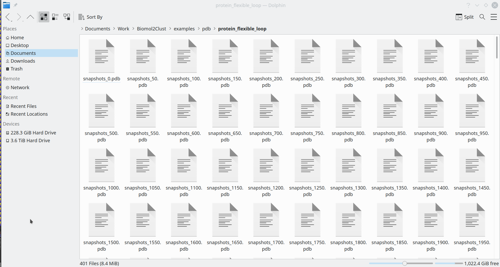
[Click here to enlarge]
- Each file should include only the object of primary interest (e.g. peptide or a protein fragment/loop region) and implement the PDB format;
- Only lines in PDB that start with the
ATOMheader will be considered for cluster analysis, i.e. the heteroatoms starting with theHETATMwill be dismissed; - The PDB input mode does not support the use of
dGdata. If you want to evaluate your conformations in association with thedGdata you should convert your PDB files to a single SDF library and use the SDF input mode, as explained above; - These separate PDB files should nevertheless preserve the common coordinate space. If opened all at once in PyMol, the viewport should reveal a biologically meaningful 3D-superimposition:
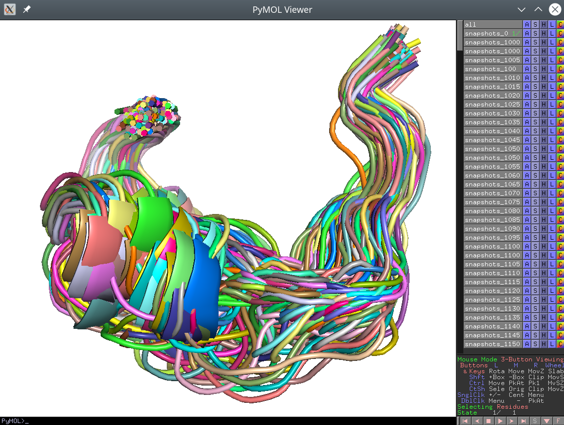
[Click here to enlarge]
- If the input conformations do not share the common coordinate space the
align=truecommand line flag should be used to attempt best-fit superimosition prior to cluster analysis.
[to the top]
Parameters
The complete list of Biomol2Clust parameters is provided below.
Mandatory input parameter
input
Default: null
Example: input=./library.sdf
Comment: Path to the input data, either the SDF library file or a folder with PDB entries.
output
Value type: string
Default: null
Example: output=./results
Comment: Path to folder to store the results.
Utilization of computing resources
cpu_threads
Value type: int
Default: all
Example: cpu_threads=10
Comment: Number of parallel CPU threads to utilize when calculating pairwise RMSD similarity matrix, and by OPTICS and DBSCAN cluster analysis. By default, RMSD similarity matrix calculations and OPTICS/DBSCAN analysis will use all physically available CPU threads. HDBSCAN can use only one thread/core of a CPU.
Cluster analysis methods
align
Value type: [true|false]
Default: false
Example: align=true
Comment: If the input conformations do not share the common coordinate space (e.g. MD shapshots were not pre-aligned), the align=true command-line switch should be used to attempt best-fit comparison prior to cluster analysis. Then, all pairs of conformations will be superimposed for best-fit prior to calculating RMSD, and the finally selected representatives of each cluster will be aligned before printing the corresponding output file.
noh
Value type: [true|false]
Default: false
Example: noh=true
Comment: Set to true to dismiss hydrogen atoms when calculating pariwise RMSD similarity matrix. The hydrogen atoms will be automatically selected based on their names: names starting from an "H" or "[number]H" will be defined as hygrogens. E.g., all these atom names "H", "H1", "HN12", "23HN" will be treated as hydrogen, while "NH1" will not be treated as one. The hydrogen atoms for each conformation will still be printed to output files. The default value is false, meaning that all atoms will be explicitly considered for RMSD calculations.
method
Value type: [hdbscan|optics|dbscan]
Default: hdbscan
Example: method=optics
Comment: Select the cluster analysis method. By default, the fully automated HDBSCAN algorithm is used to produce "thicker" clusters and minimize the amount of outliers, thus preserving as much data as possible for further expert analysis. Two alternative methods can be switched on for a particular purpose. The OPTICS is a fully automatic technique that tends to produce more spatially consistent (compact) "thinner" clusters at the cost of data loss by throwing out a larger number of proteins as outliers. Then, the DBSCAN is a curated technique dependent on the ‘eps’ parameter that can be manually calibrated to meet the particular research objective (see below).
eps
Value type: float
Default: null
Example: eps=1
Comment: Set the eps>0 to fine-tune the output of DBSCAN cluster analysis algorithm.
min_samples
Value type: int (number of conformations)
Default: when HDBSCAN is used: Null, otherwise (OPTICS, DBSCAN): 5
Example: min_samples=10
Comment: The purpose of this parameter is to regulate the minimal size of a cluster. This parameter applies to all three implemented machine learning methods: i.e. HDBSCAN, OPTICS and DBSCAN. For HDBSCAN, we recommend to use the min_cluster_size instead, see below. Formal definition of this parameter is a follows: the number of fragments of local 3D-structure in a neighborhood of the current fragment for it to be considered as the core point for clustering (the current fragment included). More information on the min_samples parameter can be found in documentation to the respective methods: the HDBSCAN parameters are explained here; the OPTICS parameters are explained here; the DBSCAN parameters are explained here, respectively.
min_cluster_size
Value type: int (number of proteins)
Default: when HDBSCAN is used: 5, otherwise (OPTICS, DBSCAN): N/A
Example: min_cluster_size=10
Comment: The purpose of this parameter is to regulate the minimal size of a cluster. This parameter applies only to HDBSCAN algorithm, and should be considered as a "better" alternative to the min_samples parameter explained above. More information about the min_cluster_size parameter can be found in the HDBSCAN documentation available here.
[to the top]
Output
Biomol2Clust produces four types of output files upon successful completion:
- Summary of the results will be printed to file
RESULTS.txt. An example of such file is provided below:
-------- ----------- ------------ ----------- ------------ ---------- -----------
Rank Сardinality Mean(energy) Std(energy) Best(energy) RMSD(mean) RMSD(stdev)
1 81 -8.441 1.277 -11.052 9.389 2.427
2 6 -8.123 0.648 -9.291 7.785 2.505
outliers 17 -7.732 0.52 -8.779 N/A N/A
-------- ----------- ------------ ----------- ------------ ---------- -----------
- Classification of input conformation into clusters and outliers will be printed to a separate file
RESULTS_cluster_content_names.txt. This file contains only the IDs/names of input conformations and their assignment to output clusters/outliers. If input conformations were provided as a single SDF file, then they will be referred to by their rank (order of appearance in the SDF library, e.g.:
Structures in cluster #1:

	6 7 8 9 10 11 12 13 14 15 16 17 18 19 20 21 22 23 24 25 26 27 28 29 30 31 32 33 34 35 36 37 38 39 40 41 97 42 43 44 45 47 48 49 50 51 52 53 54 55 56 57 58 59 60 61 62 63 64 65 66 68 70 71 72 73 74 75 76 77 78 80 82 83 84 85 86 87 88 91 92

	Structures in cluster #2:

	93 96 98 101 103 104 Outliers: 94 95 46 99 3 100 1 2 102 5 4 67 69 79 81 89 90
If input conformations were provided as separate files in PDB format, then they will be referred to by respective file names, e.g.:
Structures in cluster #1:

	snapshots_12050.pdb snapshots_8000.pdb snapshots_9950.pdb snapshots_16100.pdb snapshots_19450.pdb ...

	Structures in cluster #2:

	snapshots_5700.pdb snapshots_4250.pdb snapshots_6800.pdb snapshots_3100.pdb snapshots_4850.pdb ...

	Structures in cluster #3:

	snapshots_1100.pdb snapshots_1650.pdb snapshots_150.pdb snapshots_0.pdb snapshots_1700.pdb ...

	Outliers:

snapshots_2550.pdb snapshots_7550.pdb snapshots_50.pdb snapshots_2400.pdb snapshots_2500.pdb ... - For each cluster, a separate file is created with conformations assigned to that cluster. These files contain 3D-coordinates of input conformations, to be opened in a 3D-viewer. These files are in the same format as the input, i.e. SDF or PDB, and are named according to the cluster rank and population (as in the
RESULTS.txtfile). In additions, if thedGwas provided in the SDF library, than the mean, stddev and best (i.e. lowest) energies within the cluster will also be included into the filename, e.g.:
cluster1_size81_meandg=-8.441_bestdg=-11.052.sdf

	cluster2_size6_meandg=-8.123_bestdg=-9.291.sdf

	outliers_size17_meandg=-7.732_bestdg=-8.779.sdf
- For each cluster, a separate file is created with the "central" ("medium"/"representative") conformation of that cluster, i.e. a conformation with the lowest sum of all pairwise RMSD similarity metric within the cluster compared to all other members of that cluster. These files contain 3D-coordinates of the selected conformations, to be opened in a 3D-viewer. These files are in the same format as the input, i.e. SDF or PDB, and are named according to the cluster rank and population (as in the
RESULTS.txtfile) with the addition ofREPCONF_prefix, e.g.:
REPCONF_cluster1_size81_meandg=-8.441_bestdg=-11.052.sdf

	REPCONF_cluster2_size6_meandg=-8.123_bestdg=-9.291.sdf

	REPCONF_outliers_size17_meandg=-7.732_bestdg=-8.779.sdf
[to the top]
Examples
The distribution package of Biomol2Clust includes the source code and four types of input data to illustrate potentials of the new tool:
examples/sdf/docked_poses_with_dG.sdf- example SDF library with docked poses anddGinformation provided for each entry. The docked poses in SDF library share the common coordinate space, i.e. they were docked into the same target site of one protein structure;examples/sdf/docked_poses_no_dG.sdf- the same docked poses as explained above, but nodGinformation included;examples/pdb/protein_flexible_loop/- example PDB batch representing different conformational states of a flexible protein loop. These conformations share the common coordinate space as they were cut out from superimposed molecular dynamics snapshots of a full-size protein;examples/pdb/peptide_unaligned_conformations/- example PDB batch representing different conformational states of a cyclic peptide which were cut out from molecular dynamics snapshots but were not superimposed for best-fit. These entries do not share a common coordinate space and should be pre-aligned prior to cluster analysis using thealign=truecommand-line switch;
Example 1: Perform cluster analysis of docked poses in SDF format with dG data included into each entry
- Run the following command to cluster the SDF library using the default HDBSCAN algorithm:
python3 main.py input=examples/sdf/docked_poses_with_dG.sdf output=sdf_clusters
Please note, that the command above will explicitly consider hydrogen atoms for cluster analysis (i.e. they will be included into the RMSD calculations together with the heavy atoms). If you wish to exclude H-atoms when calculating pairwise RMSD similarity matrix, you should add thenoh=truecommand-line flag to the command above. - The output data will contain summary information for each cluster and
dGvalues of its members, and the clusters themselves in dedicated SDF files. The summaryRESULTS.txtfile will look like this:-------- ----------- ------------ ----------- ------------ ---------- -----------
Rank      Сardinality  Mean(energy)  Std(energy)  Best(energy)  RMSD(mean)  RMSD(stdev)

	1         81           -8.441        1.277        -11.052       9.389       2.427

	2         6            -8.123        0.648        -9.291        7.785       2.505

	outliers  17           -7.732        0.52         -8.779        N/A         N/A

	--------  -----------  ------------  -----------  ------------  ----------  -----------
The output clusters will be in the SDF format and the filenames will look like this:
cluster1_size81_meandg=-8.441_bestdg=-11.052.sdf

	cluster2_size6_meandg=-8.123_bestdg=-9.291.sdf

	outliers_size17_meandg=-7.732_bestdg=-8.779.sdf
- For each cluster, a separate file with the representative configuration of that cluster (i.e. a configuration with the lowest sum of pairwise RMSD similarity metric within the cluster) will be created:
REPCONF_cluster1_size81_meandg=-8.441_bestdg=-11.052.sdf
REPCONF_cluster2_size6_meandg=-8.123_bestdg=-9.291.sdf
REPCONF_outliers_size17_meandg=-7.732_bestdg=-8.779.sdf - Map the results onto the reference protein structure:
pymol examples/sdf/protein_reference.pdb `ls sdf_clusters/*sdf | sort -V`
Example 2: Perform cluster analysis of docked poses in SDF format without the dG data included
- Run the following command to cluster the SDF library using the default HDBSCAN algorithm to process the same SDF library as in the Example 1, but without the
dGincluded into each entry:
python3 main.py input=examples/sdf/docked_poses_no_dG.sdf output=sdf_clusters
Please note, that the command above will explicitly consider hydrogen atoms for cluster analysis (i.e. they will be included into the RMSD calculations together with the heavy atoms). If you wish to exclude H-atoms when calculating pairwise RMSD similarity matrix, you should add thenoh=truecommand-line flag to the command above. - The output data will contain summary information for each cluster but will not report
dGvalues of its members, and the clusters themselves in dedicated SDF files. The summaryRESULTS.txtfile will look like this:-------- ----------- ------------ ----------- ------------ ---------- -----------
Rank Сardinality Mean(energy) Std(energy) Best(energy) RMSD(mean) RMSD(stdev)
1 81 0.0 0.0 0 9.389 2.427
2 6 0.0 0.0 0 7.785 2.505
outliers 17 0.0 0.0 0 N/A N/A
-------- ----------- ------------ ----------- ------------ ---------- -----------
The output clusters will be in the SDF format and the filenames will look like this:
cluster1_size81_meandg=0.0_bestdg=0.sdf

	cluster2_size6_meandg=0.0_bestdg=0.sdf

outliers_size17_meandg=0.0_bestdg=0.sdf - For each cluster, a separate file with the representative configuration of that cluster (i.e. a configuration with the lowest sum of pairwise RMSD similarity metric within the cluster) will be created:
REPCONF_cluster1_size81_meandg=0.0_bestdg=0.sdf

	REPCONF_cluster2_size6_meandg=0.0_bestdg=0.sdf

REPCONF_outliers_size17_meandg=0.0_bestdg=0.sdf - Map the results onto the reference protein structure:
pymol examples/sdf/protein_reference.pdb `ls sdf_clusters/*sdf | sort -V`
Example 3: Perform cluster analysis of pre-aligned protein flexible loop states in PDB format
- Run the following command to cluster the PDB files that represent structural states of a flexible loop that were cut from superimposed molecular dynamics snapshots of a full-size protein using the default HDBSCAN algorithm (use can also add
noh=truecommand-line flag if you wish to dismiss hydrogen atoms from cluster analysis):
python3 main.py input=examples/pdb/protein_flexible_loop output=pdb_clusters - The output clusters will be in the SDF format and the filenames will look like this:
cluster1_size245.pdb

	cluster2_size100.pdb

	cluster3_size49.pdb

	outliers_size7.pdb
- The representative configurations for each cluster will be printed to separate files:
REPCONF_cluster1_size245.pdb

	REPCONF_cluster2_size100.pdb

	REPCONF_cluster3_size49.pdb

	REPCONF_outliers_size7.pdb
- View all clusters in PyMol:
pymol `ls pdb_clusters/*pdb | sort -V`
Example 4: Perform cluster analysis of un-aligned peptide conformational variants
- In this example, we will cluster structural states of a cyclic peptide which do not share a common coordinate space (i.e. they were not pre-aligned). Use the align=true to request pre-alignment of all pairs of conformations prior to calculation of RMSD similarity matrix (use can also add
noh=truecommand-line flag if you wish to dismiss hydrogen atoms from cluster analysis):
python3 main.py method=dbscan eps=1 input=examples/pdb/peptide_unaligned_conformations/ output=peptide_clusters align=true - The output files will contain superimposed members of each cluster (i.e. the coordinates of input and output data can differ).
Example 5: Fine-tune the output of DBSCAN cluster analysis using the eps parameter
- HDBSCAN and OPTICS allow the user to define the expected size of clusters (i.e. using
min_samplesand/ormin_cluster_sizekeywords), but otherwise are fully automatic. For a particular purpose, you can fine-tune the results of cluster analysis by playing with theepsparameter of the curated DBSCAN machine learning technique. In the example below, run Biomol2Clust with different manually calibratedepsvalues to create different clusters and outliers from the same input data:
python3 main.py method=dbscan eps=2.6 output=results align=true input=examples/pdb/peptide_unaligned_conformations/

	python3 main.py method=dbscan eps=2.8 output=results align=true input=examples/pdb/peptide_unaligned_conformations/

	python3 main.py method=dbscan eps=2.86 output=results align=true input=examples/pdb/peptide_unaligned_conformations/

	python3 main.py method=dbscan eps=2.9 output=results align=true input=examples/pdb/peptide_unaligned_conformations/

	python3 main.py method=dbscan eps=3.0 output=results align=true input=examples/pdb/peptide_unaligned_conformations/

	python3 main.py method=dbscan eps=3.1 output=results align=true input=examples/pdb/peptide_unaligned_conformations/

	python3 main.py method=dbscan eps=3.5 output=results align=true input=examples/pdb/peptide_unaligned_conformations/
[to the top]
Acknowledgments
This work was supported by the Russian Foundation for Basic Research grant #19-04-01297